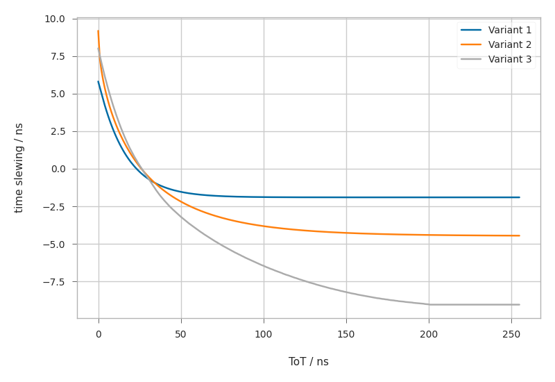
PMT Time Slewing

Show different variants of PMT time slewing calculations.

Time slewing corrects the hit time due to different rise times of the PMT signals depending on the number of photo electrons. The reference point is at 26.4ns and hits with a different ToT values are corrected to refer to comparable arrival times. The time slewing is subtracted from the measured hit time, in contrast to the time calibration (t0), which is added.

The time slewing correction is automatically applied in km3pipe when using kp.calib.Calibration().apply(), however it can be turned off by providing correct_slewing=False and also the variant can be picked by slewing_variant=X.

Variant 3 is currently (as of 2020-10-16) also used in Jpp.

# Author: Tamas Gal <tgal@km3net.de>
# License: BSD-3

import km3pipe as kp
import numpy as np
import matplotlib.pyplot as plt

kp.style.use()

tots = np.arange(256)

The kp.cali.slew() function can be used to calculate the slew. It takes a single ToT or an array of ToTs and optionally a variant. Here is the docstring of the function:

help(kp.calib.slew)

Help on function slew in module km3pipe.calib:

slew(tot, variant=3)
    Calculate the time slewing of a PMT response for a given ToT


    Parameters
    ----------
    tot: int or np.array(int)
        Time over threshold value of a hit
    variant: int, optional
        The variant of the slew calculation.
        1: The first parametrisation approach
        2: Jannik's improvement of the parametrisation
        3: The latest lookup table approach based on lab measurements.

    Returns
    -------
    time: int
        Time slewing, which has to be subtracted from the original hit time.

Calculating the slew for all variants:

slews = {variant: kp.calib.slew(tots, variant=variant) for variant in (1, 2, 3)}

fig, ax = plt.subplots()

for variant, slew in slews.items():
    ax.plot(tots, slew, label=f"Variant {variant}")

ax.set_xlabel("ToT / ns")
ax.set_ylabel("time slewing / ns")
ax.legend()

fig.tight_layout()
plt.show()