Basic Analysis Example

# Authors: Tamás Gál <tgal@km3net.de>, Moritz Lotze <mlotze@km3net.de>
# License: BSD-3
# Date: 2017-10-10
# Status: Under construction...
#
# sphinx_gallery_thumbnail_number = 5

Preparation

The very first thing we do is importing our libraries and setting up the Jupyter Notebook environment.

import matplotlib.pyplot as plt  # our plotting module
import pandas as pd  # the main HDF5 reader
import numpy as np  # must have
import km3pipe as kp  # some KM3NeT related helper functions
import seaborn as sns  # beautiful statistical plots!
from km3net_testdata import data_path

this is just to make our plots a bit “nicer”, you can skip it

import km3pipe.style

km3pipe.style.use("km3pipe")

Accessing the Data File(s)

In the following, we will work with one random simulation file with reconstruction information from JGandalf which has been converted from ROOT to HDF5 using the h5extract command line tool provided by KM3Pipe.

You can find the documentation here: https://km3py.pages.km3net.de/km3pipe/cmd.html#h5extract

Note for Lyon Users

If you are working on the Lyon cluster, you just need to load the Python module with module load python and you are all set.

Converting from ROOT to HDF5 (if needed)

Choose a file (take e.g. one from /in2p3/km3net/mc/…), load the appropriate Jpp/Aanet version and convert it via:

h5extract /path/to/a/reconstructed/file.root

You can toggle a few options to include or exclude specific information. By default, everything will be extracted but you might want to skip Example the hit information. Have a look at h5extract -h.

You might also just pick some of the already converted files from HPSS/iRODS!

First Look at the Data

filepath = data_path("hdf5/basic_analysis_sample.h5")

We can have a quick look at the file with the ptdump command in the terminal:

ptdump filename.h5

For further information, check out the documentation of the KM3NeT HDF5 format definition: http://km3pipe.readthedocs.io/en/latest/hdf5.html

The /event_info table contains general information about each event. The data is a simple 2D table and each event is represented by a single row.

Let’s have a look at the first few rows:

event_info = pd.read_hdf(filepath, "/event_info")
print(event_info.head(5))

   det_id  frame_index  livetime_sec  ...  weight_w3  run_id  event_id
0      -1            5             0  ...    0.07448       1         0
1      -1            8             0  ...    0.13710       1         1
2      -1           13             0  ...    0.11890       1         2
3      -1           15             0  ...    0.29150       1         3
4      -1           18             0  ...    0.10220       1         4

[5 rows x 17 columns]

You can easily inspect the columns/fields of a Pandas.Dataframe with the .dtypes attribute:

print(event_info.dtypes)

det_id               int32
frame_index         uint32
livetime_sec        uint64
mc_id                int32
mc_t               float64
n_events_gen        uint64
n_files_gen         uint64
overlays            uint32
trigger_counter     uint64
trigger_mask        uint64
utc_nanoseconds     uint64
utc_seconds         uint64
weight_w1          float64
weight_w2          float64
weight_w3          float64
run_id              uint64
event_id            uint32
dtype: object

And access the data either by the property syntax (if it’s a valid Python identifier) or the dictionary syntax, for example to access the neutrino weights:

print(event_info.weight_w2)  # property syntax
print(event_info["weight_w2"])  # dictionary syntax

0       1.396000e+09
1       8.907000e+09
2       5.709000e+09
3       8.747000e+10
4       3.571000e+09
            ...
3479    7.968000e+11
3480    1.736000e+09
3481    4.861000e+09
3482    7.043000e+10
3483    7.744000e+12
Name: weight_w2, Length: 3484, dtype: float64
0       1.396000e+09
1       8.907000e+09
2       5.709000e+09
3       8.747000e+10
4       3.571000e+09
            ...
3479    7.968000e+11
3480    1.736000e+09
3481    4.861000e+09
3482    7.043000e+10
3483    7.744000e+12
Name: weight_w2, Length: 3484, dtype: float64

Next, we will read out the MC tracks which are stored under /mc_tracks.

tracks = pd.read_hdf(filepath, "/mc_tracks")

It has a similar structure, but now you can have multiple rows which belong to an event. The event_id column holds the ID of the corresponding event.

print(tracks.head(10))

   bjorkeny     dir_x     dir_y     dir_z  ...   pos_z  time  type  event_id
0  0.057346 -0.616448 -0.781017 -0.100017  ... -71.802     0   -14         0
1  0.000000  0.488756 -0.535017 -0.689111  ... -71.802     0    22         0
2  0.000000 -0.656758 -0.746625 -0.105925  ... -71.802     0   -13         0
3  0.000000  0.412029 -0.878991 -0.240015  ... -71.802     0  2112         0
4  0.000000 -0.664951 -0.468928  0.581332  ... -71.802     0  -211         0
5  0.437484  0.113983  0.914457  0.388298  ...  30.360     0   -14         1
6  0.000000 -0.345462  0.923065 -0.169138  ...  30.360     0    22         1
7  0.000000  0.381285  0.828365  0.410406  ...  30.360     0   -13         1
8  0.000000 -0.191181  0.907296  0.374518  ...  30.360     0  3122         1
9  0.000000 -0.244006  0.922082  0.300377  ...  30.360     0   321         1

[10 rows x 15 columns]

We now are accessing the first track for each event by grouping via event_id and calling the first() method of the Pandas.DataFrame object.

primaries = tracks.groupby("event_id").first()

Here are the first 5 primaries:

print(primaries.head(5))

          bjorkeny     dir_x     dir_y     dir_z  ...    pos_y   pos_z  time  type
event_id                                          ...
0         0.057346 -0.616448 -0.781017 -0.100017  ...   67.589 -71.802     0   -14
1         0.437484  0.113983  0.914457  0.388298  ... -109.844  30.360     0   -14
2         0.549859 -0.186416 -0.385939 -0.903493  ...  101.459 -30.985     0    14
3         0.056390 -0.371672  0.550002 -0.747902  ...   15.056  24.474     0   -14
4         0.049141 -0.124809 -0.979083  0.160683  ...   88.981 -65.848     0    14

[5 rows x 14 columns]

Creating some Fancy Graphs

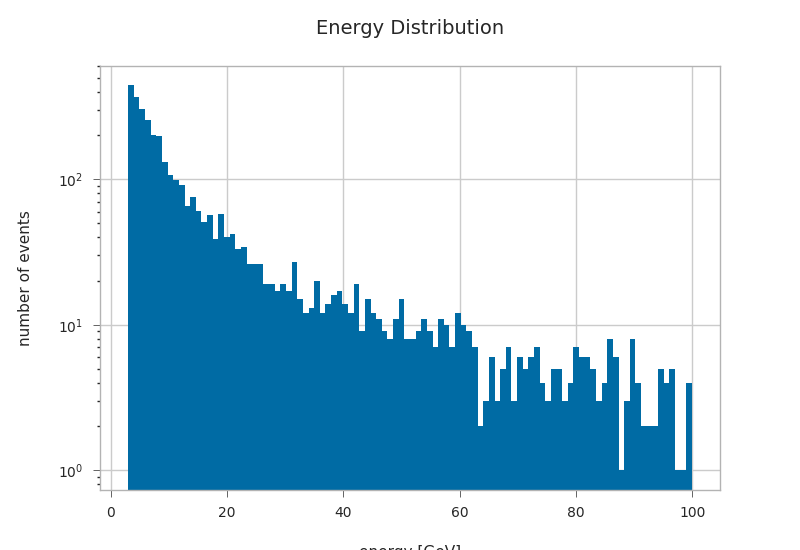
plt.hist(primaries.energy, bins=100, log=True)
plt.xlabel("energy [GeV]")
plt.ylabel("number of events")
plt.title("Energy Distribution")

Text(0.5, 1.0, 'Energy Distribution')

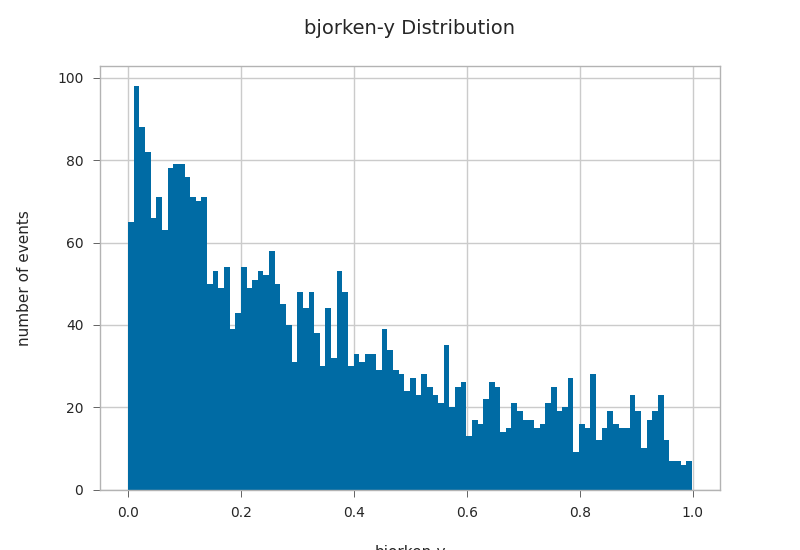
primaries.bjorkeny.hist(bins=100)
plt.xlabel("bjorken-y")
plt.ylabel("number of events")
plt.title("bjorken-y Distribution")

Text(0.5, 1.0, 'bjorken-y Distribution')

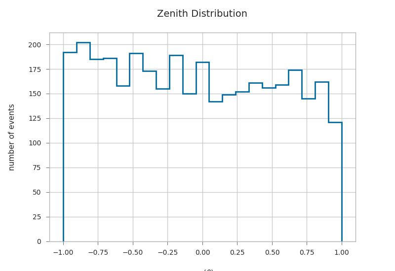
zeniths = kp.math.zenith(primaries.filter(regex="^dir_.?$"))
primaries["zenith"] = zeniths

plt.hist(np.cos(primaries.zenith), bins=21, histtype="step", linewidth=2)
plt.xlabel(r"cos($\theta$)")
plt.ylabel("number of events")
plt.title("Zenith Distribution")

Text(0.5, 1.0, 'Zenith Distribution')

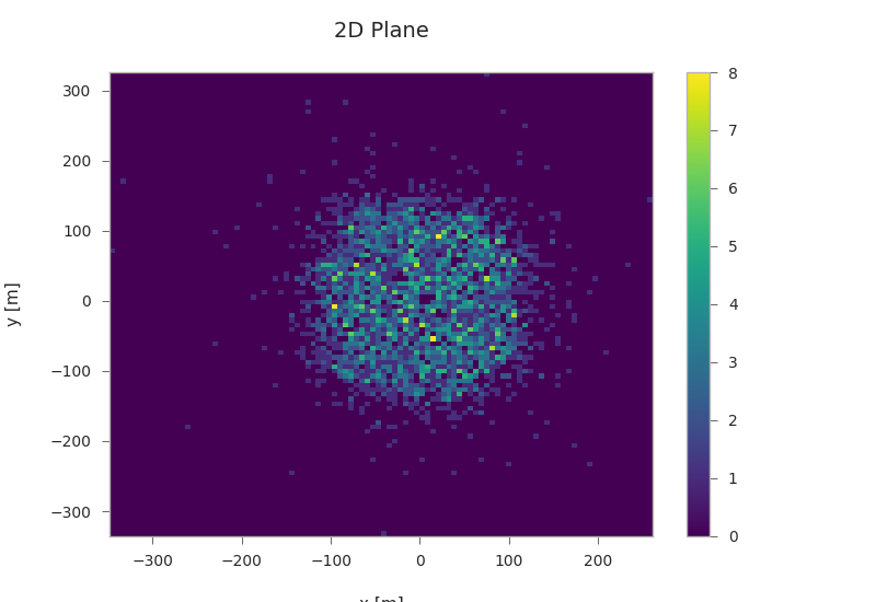
Starting positions of primaries

plt.hist2d(primaries.pos_x, primaries.pos_y, bins=100, cmap="viridis")
plt.xlabel("x [m]")
plt.ylabel("y [m]")
plt.title("2D Plane")
plt.colorbar()

<matplotlib.colorbar.Colorbar object at 0x7f35c1d49a00>

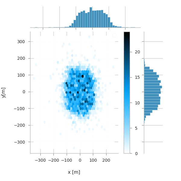
If you have seaborn installed (pip install seaborn), you can easily create nice jointplots:

try:
    import seaborn as sns  # noqa

    km3pipe.style.use("km3pipe")  # reset matplotlib style
except:
    print("No seaborn found, skipping example.")
else:
    g = sns.jointplot(x="pos_x", y="pos_y", data=primaries, kind="hex")
    g.set_axis_labels("x [m]", "y[m]")
    plt.subplots_adjust(right=0.90)  # make room for the colorbar
    plt.title("2D Plane")
    plt.colorbar()
    plt.legend()

No artists with labels found to put in legend.  Note that artists whose label start with an underscore are ignored when legend() is called with no argument.

from mpl_toolkits.mplot3d import Axes3D  # noqa

fig = plt.figure()
ax = fig.add_subplot(111, projection="3d")
ax.scatter3D(primaries.pos_x, primaries.pos_y, primaries.pos_z, s=3)
ax.set_xlabel("x [m]", labelpad=10)
ax.set_ylabel("y [m]", labelpad=10)
ax.set_zlabel("z [m]", labelpad=10)
ax.set_title("3D Plane")

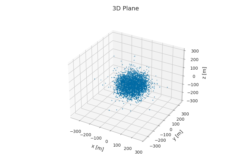
Text(0.5, 1.0, '3D Plane')

gandalfs = pd.read_hdf(filepath, "/reco/gandalf")
print(gandalfs.head(5))

      beta0     beta1        chi2  ...  type  upgoing_vs_downgoing  event_id
0  0.016788  0.011857  -53.119816  ...   0.0             -0.274836         0
1  0.007835  0.005533  -32.504874  ...   0.0              3.907941         1
2  0.012057  0.008456  -81.195134  ...   0.0             -0.385038         2
3  0.007858  0.005554 -200.985734  ...   0.0             -0.809872         3
4  0.011166  0.007366  -89.451264  ...   0.0             -0.167897         4

[5 rows x 83 columns]

gandalfs.columns

Index(['beta0', 'beta1', 'chi2', 'dir_x', 'dir_y', 'dir_z', 'jenergy_chi2',
       'jenergy_energy', 'jstart_length', 'jstart_npe_mip',
       'jstart_npe_mip_total', 'lambda', 'n_hits', 'n_iter', 'pos_x', 'pos_y',
       'pos_z', 'rec_stage', 'rec_type', 'spread_beta0_iqr',
       'spread_beta0_mad', 'spread_beta0_mean', 'spread_beta0_median',
       'spread_beta0_std', 'spread_beta1_iqr', 'spread_beta1_mad',
       'spread_beta1_mean', 'spread_beta1_median', 'spread_beta1_std',
       'spread_chi2_iqr', 'spread_chi2_mad', 'spread_chi2_mean',
       'spread_chi2_median', 'spread_chi2_std', 'spread_dir_x_iqr',
       'spread_dir_x_mad', 'spread_dir_x_mean', 'spread_dir_x_median',
       'spread_dir_x_std', 'spread_dir_y_iqr', 'spread_dir_y_mad',
       'spread_dir_y_mean', 'spread_dir_y_median', 'spread_dir_y_std',
       'spread_dir_z_iqr', 'spread_dir_z_mad', 'spread_dir_z_mean',
       'spread_dir_z_median', 'spread_dir_z_std', 'spread_jenergy_chi2_iqr',
       'spread_jenergy_chi2_mad', 'spread_jenergy_chi2_mean',
       'spread_jenergy_chi2_median', 'spread_jenergy_chi2_std',
       'spread_jenergy_energy_iqr', 'spread_jenergy_energy_mad',
       'spread_jenergy_energy_mean', 'spread_jenergy_energy_median',
       'spread_jenergy_energy_std', 'spread_n_hits_iqr', 'spread_n_hits_mad',
       'spread_n_hits_mean', 'spread_n_hits_median', 'spread_n_hits_std',
       'spread_pos_x_iqr', 'spread_pos_x_mad', 'spread_pos_x_mean',
       'spread_pos_x_median', 'spread_pos_x_std', 'spread_pos_y_iqr',
       'spread_pos_y_mad', 'spread_pos_y_mean', 'spread_pos_y_median',
       'spread_pos_y_std', 'spread_pos_z_iqr', 'spread_pos_z_mad',
       'spread_pos_z_mean', 'spread_pos_z_median', 'spread_pos_z_std', 'time',
       'type', 'upgoing_vs_downgoing', 'event_id'],
      dtype='object')

plt.hist(gandalfs[‘lambda’], bins=50, log=True) plt.xlabel(‘lambda parameter’) plt.ylabel(‘count’) plt.title(‘Lambda Distribution of Reconstructed Events’)

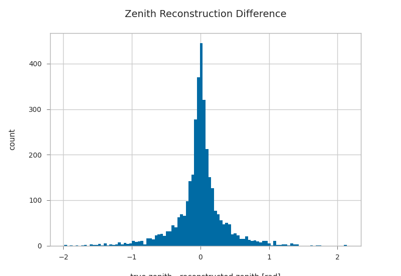
gandalfs["zenith"] = kp.math.zenith(gandalfs.filter(regex="^dir_.?$"))

plt.hist((gandalfs.zenith - primaries.zenith).dropna(), bins=100)
plt.xlabel(r"true zenith - reconstructed zenith [rad]")
plt.ylabel("count")
plt.title("Zenith Reconstruction Difference")

/builds/km3py/km3pipe/src/km3pipe/math.py:268: RuntimeWarning: invalid value encountered in divide
  unit = vector / np.linalg.norm(vector, axis=1, **kwargs)[:, None]

Text(0.5, 1.0, 'Zenith Reconstruction Difference')

l = 0.2
lambda_cut = gandalfs["lambda"] < l
plt.hist((gandalfs.zenith - primaries.zenith)[lambda_cut].dropna(), bins=100)
plt.xlabel(r"true zenith - reconstructed zenith [rad]")
plt.ylabel("count")
plt.title("Zenith Reconstruction Difference for lambda < {}".format(l))

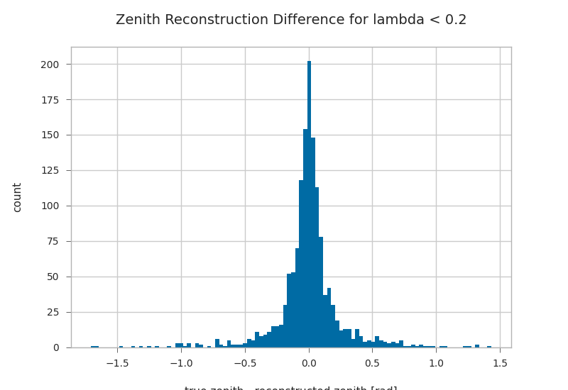
Text(0.5, 1.0, 'Zenith Reconstruction Difference for lambda < 0.2')

Combined zenith reco plot for different lambda cuts

fig, ax = plt.subplots()
for l in [100, 5, 2, 1, 0.1]:
    l_cut = gandalfs["lambda"] < l
    ax.hist(
        (primaries.zenith - gandalfs.zenith)[l_cut].dropna(),
        bins=100,
        label=r"$\lambda$ = {}".format(l),
        alpha=0.7,
    )
plt.xlabel(r"true zenith - reconstructed zenith [rad]")
plt.ylabel("count")
plt.legend()
plt.title("Zenith Reconstruction Difference for some Lambda Cuts")

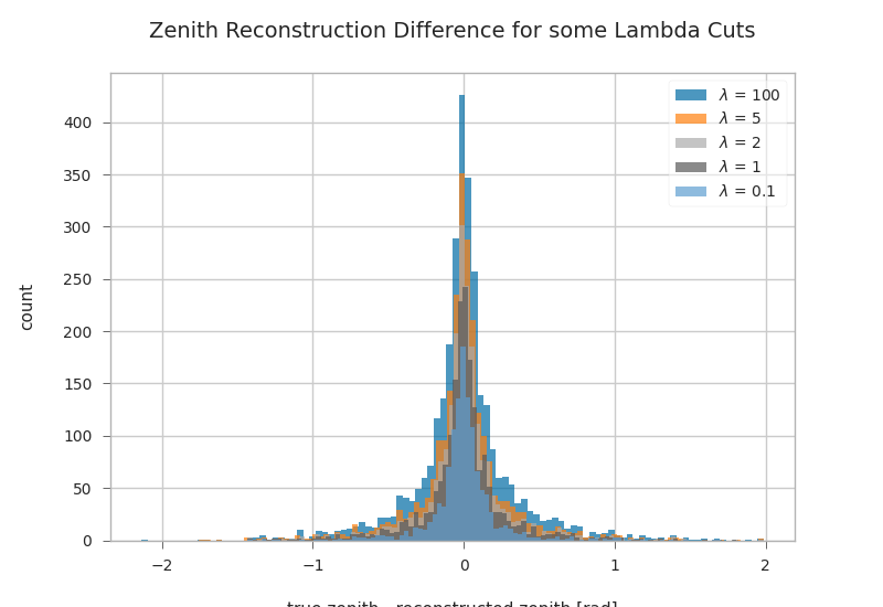
Text(0.5, 1.0, 'Zenith Reconstruction Difference for some Lambda Cuts')

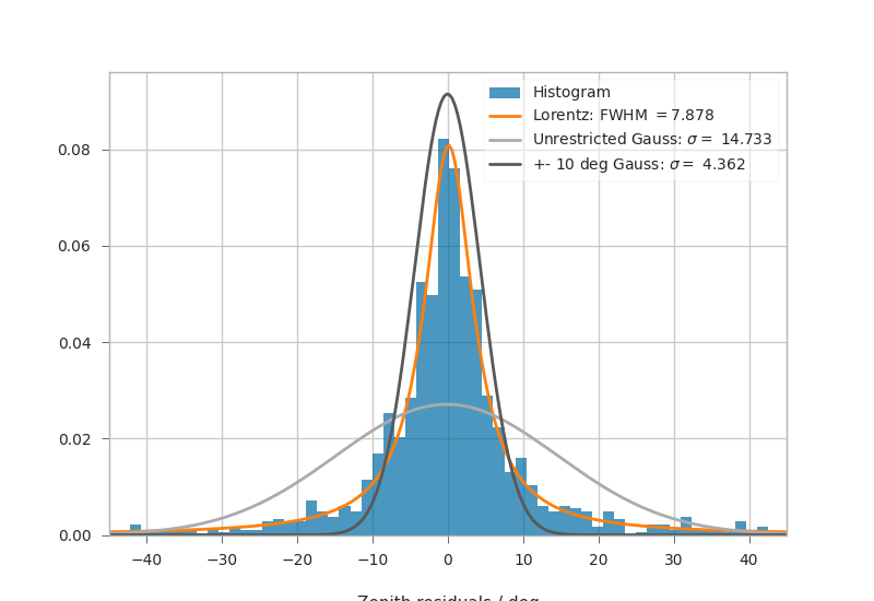
Fitting Angular resolutions

Let’s fit some distributions: gaussian + lorentz (aka norm + cauchy)

Fitting the gaussian to the whole range is a very bad fit, so we make a second gaussian fit only to +- 10 degree. Conversely, the Cauchy (lorentz) distribution is a near perfect fit (note that 2 gamma = FWHM).

from scipy.stats import cauchy, norm  # noqa

residuals = gandalfs.zenith - primaries.zenith
cut = (gandalfs["lambda"] < l) & (np.abs(residuals) < 2 * np.pi)
residuals = residuals[cut]
event_info[cut]

# convert rad -> deg
residuals = residuals * 180 / np.pi

pi = 180
# x axis for plotting
x = np.linspace(-pi, pi, 1000)

c_loc, c_gamma = cauchy.fit(residuals)
fwhm = 2 * c_gamma

g_mu_bad, g_sigma_bad = norm.fit(residuals)
g_mu, g_sigma = norm.fit(residuals[np.abs(residuals) < 10])

plt.hist(residuals, bins="auto", label="Histogram", density=True, alpha=0.7)
plt.plot(
    x,
    cauchy(c_loc, c_gamma).pdf(x),
    label="Lorentz: FWHM $=${:.3f}".format(fwhm),
    linewidth=2,
)
plt.plot(
    x,
    norm(g_mu_bad, g_sigma_bad).pdf(x),
    label="Unrestricted Gauss: $\sigma =$ {:.3f}".format(g_sigma_bad),
    linewidth=2,
)
plt.plot(
    x,
    norm(g_mu, g_sigma).pdf(x),
    label="+- 10 deg Gauss: $\sigma =$ {:.3f}".format(g_sigma),
    linewidth=2,
)
plt.xlim(-pi / 4, pi / 4)
plt.xlabel("Zenith residuals / deg")
plt.legend()

<matplotlib.legend.Legend object at 0x7f35c110f730>

We can also look at the median resolution without doing any fits.

In textbooks, this metric is also called Median Absolute Deviation.

resid_median = np.median(residuals)
residuals_shifted_by_median = residuals - resid_median
absolute_deviation = np.abs(residuals_shifted_by_median)
resid_mad = np.median(absolute_deviation)

plt.hist(np.abs(residuals), alpha=0.7, bins="auto", label="Absolute residuals")
plt.axvline(resid_mad, label="MAD: {:.2f}".format(resid_mad), linewidth=3)
plt.title("Average resolution: {:.3f} degree".format(resid_mad))
plt.legend()
plt.xlabel("Absolute zenith residuals / deg")

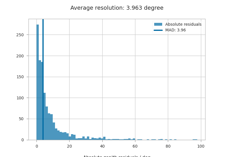
Text(0.5, 4.833333333333329, 'Absolute zenith residuals / deg')