Convex Hull

Convex hull of a set of points, representing Dom x-y positions.

Derived from scipy.spatial.qhull.pyx.

import numpy as np
from scipy.spatial import ConvexHull
import matplotlib.pyplot as plt
from mpl_toolkits.mplot3d import Axes3D  # noqa
from km3net_testdata import data_path

from km3pipe.hardware import Detector
from km3pipe.math import Polygon
import km3pipe.style

km3pipe.style.use("km3pipe")

detx = data_path(
    "detx/orca_115strings_av23min20mhorizontal_18OMs_alt9mvertical_v1.detx"
)
detector = Detector(detx)
xy = detector.xy_positions
hull = ConvexHull(xy)

Detector: Parsing the DETX header
Detector: Reading PMT information...
Detector: Done.

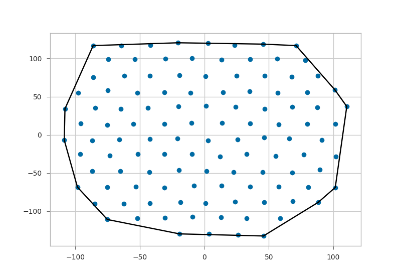
Plot it:

plt.plot(xy[:, 0], xy[:, 1], "o")
for simplex in hull.simplices:
    plt.plot(xy[simplex, 0], xy[simplex, 1], "k-")

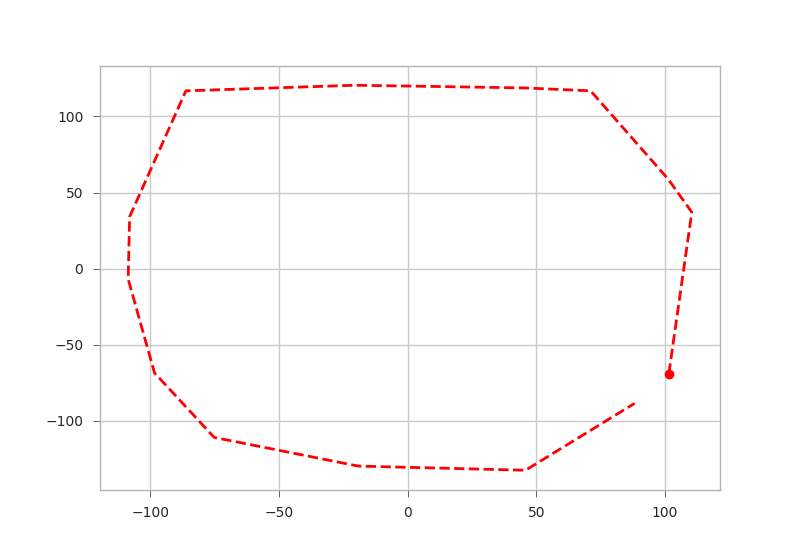
We could also have directly used the vertices of the hull, which for 2-D are guaranteed to be in counterclockwise order:

plt.plot(xy[hull.vertices, 0], xy[hull.vertices, 1], "r--", lw=2)
plt.plot(xy[hull.vertices[0], 0], xy[hull.vertices[0], 1], "ro")
plt.show()

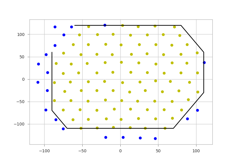
Now let’s draw a polygon inside, and see which points are contained.

poly_vertices = np.array(
    [
        (-60, 120),
        (80, 120),
        (110, 60),
        (110, -30),
        (70, -110),
        (-70, -110),
        (-90, -70),
        (-90, 60),
    ]
)
poly = Polygon(poly_vertices)
contain_mask = poly.contains(xy)

and color them accordingly

plt.clf()
plt.plot(xy[contain_mask, 0], xy[contain_mask, 1], "yo")
plt.plot(xy[~contain_mask, 0], xy[~contain_mask, 1], "bo")
plt.plot(poly_vertices[:, 0], poly_vertices[:, 1], "k-")
plt.show()

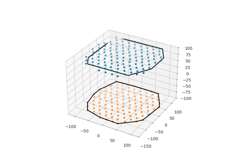
plot the same in 3D because why not?

plt.clf()
fig = plt.figure()
ax = fig.add_subplot(111, projection="3d")
ax.scatter(xy[:, 0], xy[:, 1], 90, "yo")
ax.scatter(xy[:, 0], xy[:, 1], -90, "bo")
ax.plot(poly_vertices[:, 0], poly_vertices[:, 1], 90, "k-")
for simplex in hull.simplices:
    ax.plot(xy[simplex, 0], xy[simplex, 1], -90, "k-")
plt.show()

• 
•