How to use self calibration module

The magnetic field read by the sensors inside km3net DOM are sending a measurement in cartesian referential. When a DOM is placed under an uniform magnetic field, rotating it should only results in a modification of the magnetic field direction. However, the natural coordinates system is often not centered on (0,0,0), which raise the need to perform a calibration before using converting the magnetic field data in a direction measurement.

This script is an example on how use the calib_self_sphere class on acceptance tests data in order to estimate the point around which the magnetic field is revolving, allowing a calibration directly computed on data.

import km3compass as kc
import matplotlib.pyplot as plt

Loading some data

Initialising is a simple as this:

filename = "../tests/DOM_0801.csk"
reader = kc.readerCSK(filename)
print(reader.module_IDs)

File loaded, 2508 rows
        1 module(s)
        - 817302522
Number of measurements after removing duplicates : 252
[817302522]

Loading the module

The calib_self_sphere will fit a sphere to the raw magnetic field data, and will then correct the data from the estimated center.

calib = kc.calib_self_sphere(reader, 817302522)

Print fit results

Here, we print the center and radius reconstructed by the fit. We also display a plot that summarize the calibration results.

print("Center : {}".format(calib.center.flatten()))
print("Radius : {}".format(calib.radius))
calib.plot_results()

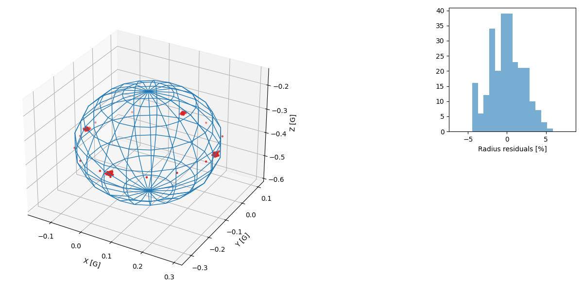
Center : [ 0.0736884  -0.10788356 -0.37211751]
Radius : [0.21029674]

Comparing data before and after calibration

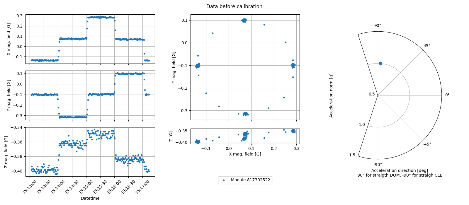
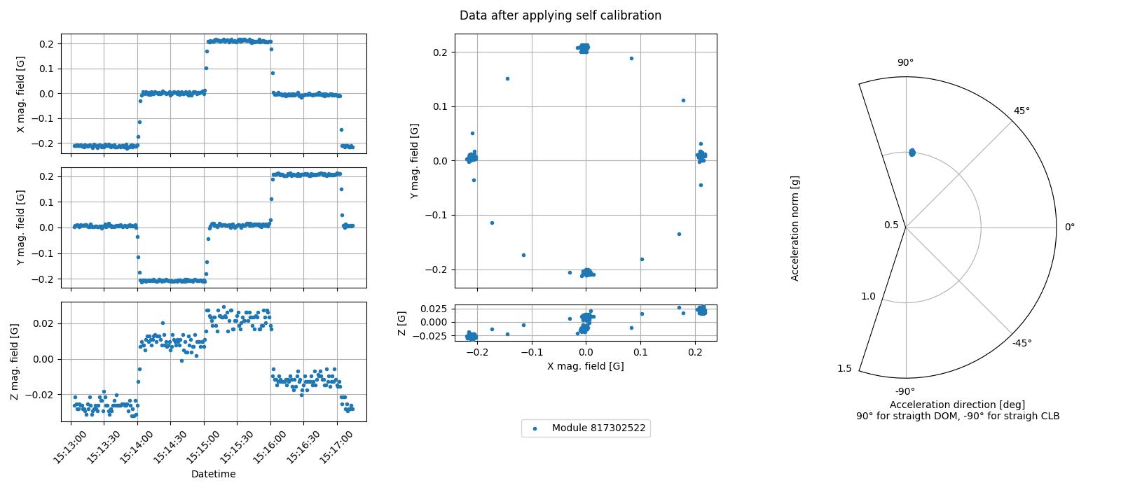
To do so, we will use the kc.plot_raw_results function, that works for both raw and calibrated data :

kc.plot_raw_results(reader.df, title="Data before calibration")

kc.plot_raw_results(calib.df, title="Data after applying self calibration")


plt.show()

• 
•